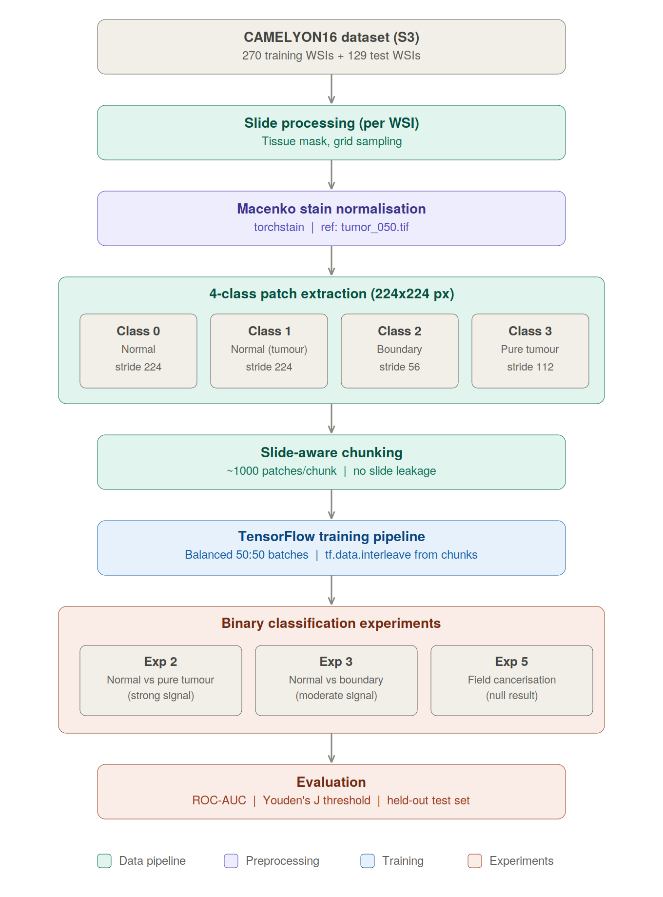
Automated Tumour Detection in Whole Slide Images: An End-to-End Deep Learning Pipeline
A practical guide to building a supervised deep learning system for detecting breast cancer metastases in histopathology images, using the CAMELYON16 challenge dataset.
Table of Contents
- 1. The Problem: Pathologist Shortages and the Promise of Automation
- 2. The CAMELYON16 Challenge
- 3. Running the code
- 4. Understanding Whole Slide Images
- 5. Step 1: Finding the Tissue
- 6. Step 2: Parsing Tumour Annotations and the Four-Class Labelling Scheme
- 7. Step 3: Building the Training Dataset
- 8. Step 4: The Training Pipeline
- 9. Step 5: Model Architecture
- 10. Step 6: Training
- 11. Step 7: Test Set Evaluation
- 12. Results
- 13. Investigating the Field Cancerisation Hypothesis
- 14. Lessons Learned
- 15. Conclusion
1. The Problem: Pathologist Shortages and the Promise of Automation
Diagnosing cancer from tissue biopsies remains one of the most critical and labour-intensive tasks in modern medicine. A pathologist examining a sentinel lymph node biopsy must scan an entire tissue section at high magnification, searching for clusters of cancer cells that may occupy only a tiny fraction of the slide. In busy services, pathologists frequently face large daily caseloads under considerable time pressure.
The numbers tell a sobering story. In the UK, the Royal College of Pathologists has warned of a sustained workforce crisis, with shortfalls reaching up to 30% in some specialties. In the US, the situation is similar: an ageing workforce, rising case volumes, and growing molecular testing demands all strain an already stretched system.
Meanwhile, the digitisation of histopathology is accelerating. Whole Slide Imaging (WSI) scanners now capture tissue sections at resolutions exceeding 100,000 × 100,000 pixels in images that capture cellular-level detail across an entire tissue section. This creates an opportunity: if we can train machine learning models to analyse these images, we can augment pathologists' workflows, flag suspicious regions for closer review, and potentially catch metastases that might be missed under time pressure.
A more speculative research question is whether models can detect subtle alterations in histologically normal-appearing tissue from tumour-bearing slides, potentially reflecting field cancerisation or other tumour-associated microenvironmental changes.
In this post, I build an end-to-end pipeline from raw whole-slide images to trained classifiers, and test how far these ideas hold up in practice. Here's an overview of the complete pipeline:
2. The CAMELYON16 Challenge
The CAMELYON16 Grand Challenge was organised in 2015–2016 by the International Symposium on Biomedical Imaging (ISBI) to benchmark automated detection of breast cancer metastases in whole slide images of sentinel lymph node biopsies.
The dataset consists of nearly 400 H&E-stained whole slide images from two Dutch medical centres (Radboud UMC and University Medical Centre Utrecht):
| Split | Tumour slides | Normal slides | Total |
|---|---|---|---|
| Train | 110 | 160 | 270 |
| Test | 49 | 80 | 129 |
Each tumour slide comes with XML annotation files containing polygon outlines of metastatic regions, hand-drawn by expert pathologists.
The winning team (Wang et al., 2016) achieved a slide-level AUC of 0.925 using a GoogLeNet-based patch classifier trained on millions of patches. Remarkably, when the system’s predictions were combined with a pathologist’s review, the pathologist’s AUC increased from 0.966 to 0.995, corresponding to an approximately 85% reduction in error.
My approach follows the same fundamental strategy (patch-based classification) but with one important modification: I introduce a four-class labelling scheme that lets me ask more nuanced questions about what the model is capable of actually detecting.
3. Running the code
This article shows the full notebook narrative and code, but the project is structured as a modular repository rather than a single standalone notebook. In Google Colab, run the next two setup cells first: one clones the repo into the runtime, and the other mounts Google Drive and checks for the pre-generated dataset.
Sections 4-7 can run directly and download slides from Amazon S3 on demand. Sections 10-12 require the pre-generated patch dataset, which you can create using the code in Section 7 (~6-8 hours generation time on Colab) or replace with your own dataset paths.
Note: Training dataset generation and model training usually require Colab Pro (High RAM) to avoid out-of-memory crashes. All other sections should run on the free tier.
# === SECTION 1: SET UP THE PROJECT CODE ===
from pathlib import Path
import os
REPO_URL = 'https://github.com/balintstewart77/camelyon16-pathology.git'
REPO_DIR = Path('/content/camelyon16-pathology')
if not REPO_DIR.exists():
!git clone {REPO_URL} /content/camelyon16-pathology
else:
print("Repository already present in runtime.")
os.chdir(REPO_DIR)
print("Current working directory:", os.getcwd())
!apt-get install -y openslide-tools > /dev/null 2>&1
!pip install -q -r requirements.txt
print("Project environment ready.")
Cloning into '/content/camelyon16-pathology'... remote: Enumerating objects: 748, done. remote: Counting objects: 100% (64/64), done. remote: Compressing objects: 100% (45/45), done. remote: Total 748 (delta 40), reused 38 (delta 19), pack-reused 684 (from 2) Receiving objects: 100% (748/748), 85.68 MiB | 49.90 MiB/s, done. Resolving deltas: 100% (486/486), done. Current working directory: /content/camelyon16-pathology ━━━━━━━━━━━━━━━━━━━━━━━━━━━━━━━━━━━━━━━━ 4.3/4.3 MB 52.8 MB/s eta 0:00:00 ━━━━━━━━━━━━━━━━━━━━━━━━━━━━━━━━━━━━━━━━ 140.5/140.5 kB 16.6 MB/s eta 0:00:00 ━━━━━━━━━━━━━━━━━━━━━━━━━━━━━━━━━━━━━━━━ 15.0/15.0 MB 127.9 MB/s eta 0:00:00 ━━━━━━━━━━━━━━━━━━━━━━━━━━━━━━━━━━━━━━━━ 86.8/86.8 kB 9.3 MB/s eta 0:00:00 Project environment ready.
# === SECTION 2: MOUNT GOOGLE DRIVE AND LOCATE THE DATASET ===
from pathlib import Path
from google.colab import drive
drive.mount('/content/drive')
# Add the shared Google Drive folder as a shortcut to your Drive:
# https://drive.google.com/drive/folders/1Ny8zXjBPsrqSFUD61v02EHsjAwgGSY47?usp=drive_link
# Right-click → "Add shortcut to Drive", place it under "My Drive",
# and name it exactly: camelyon16_data
expected_train = 'camelyon16_4class_stain_normalised'
expected_test = 'camelyon16_test_stain_normalised'
candidate_roots = [
Path('/content/drive/MyDrive/camelyon16_data'),
Path('/content/drive/MyDrive/new_work/Projects/pathovis_project/data'),
]
DATA_ROOT = None
TRAIN_PATH = None
TEST_PATH = None
for root in candidate_roots:
train_path = root / expected_train
test_path = root / expected_test
if train_path.exists() and test_path.exists():
DATA_ROOT = root
TRAIN_PATH = train_path
TEST_PATH = test_path
break
if DATA_ROOT is None:
print("Checked candidate dataset roots:")
for root in candidate_roots:
print(f"\n{root}")
print(f" exists: {root.exists()}")
if root.exists():
print(" contents:")
for child in sorted(root.iterdir())[:20]:
print(f" - {child.name}")
raise FileNotFoundError(
"Could not find the CAMELYON16 dataset.\n\n"
"Please add the shared Google Drive folder as a shortcut to your Drive:\n"
" https://drive.google.com/drive/folders/1Ny8zXjBPsrqSFUD61v02EHsjAwgGSY47?usp=drive_link\n\n"
"Steps:\n"
" 1. Open the link above\n"
" 2. Right-click the folder \u2192 'Add shortcut to Drive'\n"
" 3. Place it directly under 'My Drive'\n"
" 4. Name it exactly: camelyon16_data\n\n"
"Expected subfolders:\n"
f" - {expected_train}\n"
f" - {expected_test}"
)
print("Dataset paths verified.")
print(f"DATA_ROOT = {DATA_ROOT}")
print(f"TRAIN_PATH = {TRAIN_PATH}")
print(f"TEST_PATH = {TEST_PATH}")
Mounted at /content/drive Dataset paths verified. DATA_ROOT = /content/drive/MyDrive/new_work/Projects/pathovis_project/data TRAIN_PATH = /content/drive/MyDrive/new_work/Projects/pathovis_project/data/camelyon16_4class_stain_normalised TEST_PATH = /content/drive/MyDrive/new_work/Projects/pathovis_project/data/camelyon16_test_stain_normalised
import numpy as np
import matplotlib.pyplot as plt
import openslide
np.random.seed(42)
# Project imports
from config import DEFAULT_CONFIG
from src.data import list_s3_files, download_file_from_s3, cleanup_file
from src.data.tissue_mask import get_tissue_mask, compute_foreground_mask
from src.data.tumor_polygons import load_tumor_polygons, classify_patch
from src.data.patch_extraction import (
sample_grid_coordinates, sample_coordinates_by_class,
extract_patch, preprocess_patch,
get_stain_normaliser, normalise_stain
)
from src.visualisation import (
visualise_tissue_outline, visualise_patches_grid,
find_zoom_region_by_coords, find_dense_tissue_region
)
# Example slide used throughout the notebook's tumor-slide walkthrough.
# Changing this allows you to explore a different example normal or tumor slide
# Some clear example tumor slides nicely showing all three classes include 5,11,13,16,18,22,24,25,27,29,32,37,38,50,51,52,56,62,73,91,92,93,94,100,106,107,109,110,111
EXAMPLE_TUMOR_SLIDE_ID = 'tumor_016'
EXAMPLE_TUMOR_SLIDE = f'{EXAMPLE_TUMOR_SLIDE_ID}.tif'
EXAMPLE_TUMOR_ANNOTATION = f'{EXAMPLE_TUMOR_SLIDE_ID}.xml'
print("All imports successful!")
All imports successful!
4. Understanding Whole Slide Images
A WSI is not a regular image. At full resolution, a single slide can be over 100,000 × 100,000 pixels (roughly 60 gigabytes of uncompressed pixel data). Given its size, you cannot load one directly into memory.
Instead, many whole-slide images are stored as pyramidal tiled images often in TIFF-based formats, with the same slide saved at multiple resolutions. Using OpenSlide, you can navigate this pyramid and read small regions on demand rather than loading the entire gigapixel file into memory.
Below we download a single slide and explore its structure.
# List available slides from S3
all_slides = list_s3_files(DEFAULT_CONFIG.data.s3_images, '.tif')
normal_slides = sorted([f for f in all_slides if 'normal' in f.lower()])
tumor_slides = sorted([f for f in all_slides if 'tumor' in f.lower()])
print(f"Dataset: {len(normal_slides)} normal slides, {len(tumor_slides)} tumour slides")
print(f"\nExample normal slide: {normal_slides[0]}")
print(f"Example tumour slide: {tumor_slides[0]}")
Dataset: 159 normal slides, 111 tumour slides Example normal slide: normal_001.tif Example tumour slide: tumor_001.tif
# Download one tumour slide to explore
slide_name = EXAMPLE_TUMOR_SLIDE
slide_path = download_file_from_s3(
DEFAULT_CONFIG.data.s3_images, slide_name, '/tmp'
)
slide = openslide.OpenSlide(slide_path)
# Explore the pyramid structure
print(f"Slide: {slide_name}")
print(f"Dimensions (level 0): {slide.dimensions[0]:,} × {slide.dimensions[1]:,} pixels")
print(f"Number of levels: {slide.level_count}")
print(f"\nPyramid levels:")
for i in range(slide.level_count):
w, h = slide.level_dimensions[i]
ds = slide.level_downsamples[i]
print(f" Level {i}: {w:>7,} × {h:>7,} (downsample: {ds:.1f}×)")
Downloading tumor_016.tif... Slide: tumor_016.tif Dimensions (level 0): 97,792 × 221,184 pixels Number of levels: 10 Pyramid levels: Level 0: 97,792 × 221,184 (downsample: 1.0×) Level 1: 48,896 × 110,592 (downsample: 2.0×) Level 2: 24,448 × 55,296 (downsample: 4.0×) Level 3: 12,224 × 27,648 (downsample: 8.0×) Level 4: 6,112 × 13,824 (downsample: 16.0×) Level 5: 3,056 × 6,912 (downsample: 32.0×) Level 6: 1,528 × 3,456 (downsample: 64.0×) Level 7: 764 × 1,728 (downsample: 128.0×) Level 8: 382 × 864 (downsample: 256.0×) Level 9: 191 × 432 (downsample: 512.0×)
# View the whole slide as a thumbnail
thumbnail = slide.get_thumbnail((800, 800))
fig, ax = plt.subplots(figsize=(8, 8))
ax.imshow(thumbnail)
ax.set_title(f'{slide_name}: Thumbnail', fontsize=14)
ax.axis('off')
plt.tight_layout()
plt.show()
print(f"\nThe thumbnail is {thumbnail.size[0]}×{thumbnail.size[1]} pixels.")
print(f"The actual slide is {slide.dimensions[0]:,}×{slide.dimensions[1]:,} pixels.")
print(f"That's a {slide.dimensions[0] // thumbnail.size[0]:,}× reduction!")

The thumbnail is 354×800 pixels. The actual slide is 97,792×221,184 pixels. That's a 276× reduction!
5. Step 1: Finding the Tissue
Most of a whole-slide image is background rather than tissue. Before extracting patches, we need to identify where tissue is present so that sampling is restricted to informative regions.
Design Decision: Why Work at Thumbnail Resolution?
At full resolution, a single slide may be around 100,000 × 200,000 pixels. For the purpose of locating tissue, however, scanning the full-resolution image is unnecessary because the coarse tissue layout is already visible at much lower magnification. A 512 × 512 thumbnail can be generated quickly by OpenSlide and contains all that's needed for this step.
The tissue mask is computed on a thumbnail and used only to propose candidate patch coordinates. The classifier itself operates on full-resolution RGB patches, so these thumbnail-space coordinates must be mapped back to the original slide. get_scaling_factors() performs that mapping using the ratio between slide dimensions and mask dimensions.
scale_x = slide_width / mask_width
scale_y = slide_height / mask_height
thumbnail pixel (col, row)
↓ × scale_x, × scale_y
patch centre (x, y) in level-0 (full resolution) slide coordinates
↓ openslide.read_region(location=(x - 112, y - 112), level=0, size=(224, 224))
full-resolution 224 × 224 patch
This coarse-detection / fine-extraction workflow is standard in computational pathology. sample_grid_coordinates() follows this sequence: iterate over mask pixels, check for tissue, map coordinates back to the full-resolution slide, then extract the patch.
Design Decision: Why So Many Cleanup Steps?
Greyscale thresholding works in H&E thumbnails because tissue stains pink/purple and is usually darker than the white glass background. But a single threshold applied to a raw thumbnail produces a noisy mask with imaging artefacts (such as the border artefacts visible in tumor_005 thumbnail above). compute_foreground_mask() applies a deliberate chain of operations to handle each failure mode:
| Step | Operation | What it removes |
|---|---|---|
Threshold < 180 |
- | Selects all dark pixels |
remove_small_objects() |
min_size=100 |
Dust specks, fibres, staining dots |
clear_border() |
- | Any blob touching the image edge (scanner margins are often dark) |
remove_small_holes() |
area_threshold=100 |
Small voids within tissue blobs caused by pale staining |
| Border zeroing | border_margin=5 |
Residual edge artefacts that survive clear_border() |
filter_valid_components() then applies a second filtering pass over the remaining connected components using two criteria: minimum area and maximum aspect ratio. I include an aspect ratio filter because a thin horizontal scanner artefact may have a large pixel area while still having an extreme aspect ratio (for example 10:1), making it unlikely to be genuine tissue. The code rejects any blob exceeding max_aspect_ratio=5.0.
Cleanup order matters. clear_border() must run before filter_valid_components(). If a border artefact is not removed first, it may be joined to real tissue by a thin pixel bridge and survive as a huge elongated blob.
This sequential process illustrates a broader principle in image segmentation pipelines. Rather than relying on a single operation, these pipelines usually consist of a chain of heuristics, each handling a specific issue. The steps taken in compute_foreground_mask() and filter_valid_components() are a practical response to common WSI artefacts, crafted specifically for this use-case (in my case, mostly via a process of trial and error).
Under the Hood: Tissue Masking
The tissue masking logic is surprisingly simple. Here's what compute_foreground_mask does with just ~10 lines of core logic:
# === What compute_foreground_mask does internally ===
from skimage.morphology import remove_small_objects, remove_small_holes
from skimage.segmentation import clear_border
# Step 1: Get a tiny thumbnail (512×512) from the gigapixel image
thumbnail_gray = slide.get_thumbnail((512, 512)).convert("L")
thumbnail_array = np.array(thumbnail_gray)
# Step 2: Simple brightness threshold
# Tissue is darker than the white glass background
threshold = 180 # pixels darker than this are tissue
raw_mask = thumbnail_array < threshold
# Step 3: Morphological cleanup
cleaned = remove_small_objects(raw_mask, min_size=100) # remove dust specks
cleaned = clear_border(cleaned) # remove edge artifacts
cleaned = remove_small_holes(cleaned, area_threshold=100) # fill 'holes' in tissue (likely real tissue)
print(f"Raw mask pixels: {raw_mask.sum():,}")
print(f"After cleanup: {cleaned.sum():,}")
print(f"Removed {raw_mask.sum() - cleaned.sum():,} artifact pixels")
fig, axes = plt.subplots(1, 3, figsize=(15, 4))
axes[0].imshow(thumbnail_array, cmap='gray')
axes[0].set_title('Grayscale thumbnail')
axes[1].imshow(raw_mask, cmap='gray')
axes[1].set_title(f'After threshold (<{threshold})')
axes[2].imshow(cleaned, cmap='gray')
axes[2].set_title('After morphological cleanup')
for ax in axes: ax.axis('off')
plt.tight_layout()
plt.show()
Raw mask pixels: 5,436 After cleanup: 5,041 Removed 395 artifact pixels

# Generate tissue mask
mask = compute_foreground_mask(slide)
print(f"Mask shape: {mask.shape}")
print(f"Tissue coverage: {mask.sum() / mask.size:.1%}")
# Visualise: original thumbnail vs. detected tissue
fig, axes = plt.subplots(1, 3, figsize=(18, 6))
# Original
axes[0].imshow(thumbnail)
axes[0].set_title('Original Slide', fontsize=13)
axes[0].axis('off')
# Binary mask
axes[1].imshow(mask, cmap='gray')
axes[1].set_title('Tissue Mask', fontsize=13)
axes[1].axis('off')
# Overlay: tissue outline on slide
axes[2].imshow(thumbnail)
# Resize mask to match thumbnail
from PIL import Image
mask_resized = np.array(
Image.fromarray(mask.astype(np.uint8) * 255).resize(thumbnail.size, Image.NEAREST)
) > 127
axes[2].contour(mask_resized.astype(float), levels=[0.5], colors='lime', linewidths=1.5)
axes[2].set_title('Tissue Detection Overlay', fontsize=13)
axes[2].axis('off')
plt.tight_layout()
plt.show()
Mask shape: (512, 226) Tissue coverage: 4.4%

6. Step 2: Parsing Tumour Annotations and the Four-Class Labelling Scheme
For tumour slides, CAMELYON16 provides XML files with polygon annotations tracing the tumour boundaries. I parse these into Shapely geometry objects, which lets me compute precise overlap between any patch and the annotated tumour regions.
Design Decision: Labels come from tumour annotation geometry rather than slide identity
For tumour slides, patch labels are assigned from the geometric overlap between the 224 × 224 patch and the annotated tumour regions.
The process inside classify_patch():
- The patch centre
(x, y)is converted to ashapely.box- a rectangle in level-0 (full resolution) slide coordinate space. calculate_tumor_overlap()iterates over all tumour polygons, summing the intersection area between the patch box and each polygon.- That total is divided by the patch area (224²) to get an overlap fraction in [0, 1].
- Threshold rules from
config.pyassign the class label:
if overlap < zero_tolerance: label = 1 # Normal tissue (tumour slide)
elif overlap < tumor_threshold: label = 2 # Boundary tumour
else: label = 3 # 'Pure' tumour
For tumour slides, the label depends on the fraction of the 224 × 224 patch covered by annotated tumour. Patches with essentially zero overlap are labelled normal_from_tumor (class 1), patches with partial overlap are labelled boundary_tumor (class 2), and patches with at least 50% tumour overlap are labelled pure_tumor (class 3). The thresholds are defined explicitly in config.py, which makes the labelling reproducible and auditable.
Class 0 (normal_from_normal) is assigned separately to patches from slides with no tumour annotation file.
Design Decision: Repairing Invalid Polygon Geometry
Real annotation data is not always perfectly clean. Some CAMELYON16 XML outlines contain invalid or self-intersecting polygon geometry, so load_tumor_polygons() repairs these with Shapely before using them in overlap calculations.
The Four-Class Scheme
The pipeline uses a four-class labelling scheme based on each patch’s spatial relationship to the tumour:
| Class | Name | Description |
|---|---|---|
| 0 | normal_from_normal |
Normal tissue from a slide with no tumour at all |
| 1 | normal_from_tumor |
Normal-looking tissue on a slide that also contains tumour |
| 2 | boundary_tumor |
Tissue at the tumour margin (partial overlap with annotations) |
| 3 | pure_tumor |
Tissue fully within annotated tumour regions |
Separating classes 0 and 1 is a key scientific choice in this project. Class 1 patches may look very similar to class 0 under the microscope, but they come from tumour-bearing slides. If a model can distinguish them, it may be picking up subtle tumour-associated context, potentially including field cancerisation, stromal response, inflammatory change, or slide-level artefacts. This distinction forms the basis of Experiment 3.
This scheme lets me ask more interesting questions than simple binary classification. In particular, Class 1 vs. Class 0 tests whether normal-looking tissue from tumour-bearing slides differs detectably from tissue on tumour-free slides.
# Load tumor annotations
xml_path = download_file_from_s3(
DEFAULT_CONFIG.data.s3_annotations, EXAMPLE_TUMOR_ANNOTATION, '/tmp'
)
polygons = load_tumor_polygons(xml_path)
print(f"Loaded {len(polygons)} tumor polygons")
for i, p in enumerate(polygons):
print(f" Polygon {i}: area = {p.area:,.0f} pixels², "
f"bounds = {tuple(int(x) for x in p.bounds)}")
Downloading tumor_016.xml... Loaded 10 tumor polygons Polygon 0: area = 43,916,526 pixels², bounds = (37670, 148815, 45746, 156110) Polygon 1: area = 86,410 pixels², bounds = (38997, 158449, 39629, 158802) Polygon 2: area = 67,783 pixels², bounds = (35418, 160397, 35673, 160736) Polygon 3: area = 75,177 pixels², bounds = (30817, 160676, 31188, 161036) Polygon 4: area = 76,608 pixels², bounds = (30382, 160876, 30701, 161229) Polygon 5: area = 70 pixels², bounds = (35182, 156414, 35198, 156425) Polygon 6: area = 265,080 pixels², bounds = (35142, 156425, 35657, 157205) Polygon 7: area = 193,961 pixels², bounds = (46975, 160543, 47697, 160991) Polygon 8: area = 2,183,626 pixels², bounds = (43413, 159341, 46757, 160954) Polygon 9: area = 1 pixels², bounds = (45918, 160917, 45922, 160917)
# Visualise tumor annotations overlaid on the tissue
visualise_tissue_outline(
slide, mask,
tumor_polygons=polygons,
title='Tumor Annotations (red) with Tissue Outline (green)',
figsize=(10, 10)
)

Classifying Patches by Tumour Overlap
Each patch is classified by computing the fractional overlap between the 224×224 patch and the tumour polygons:
- < 1% overlap → Class 1 (normal tissue on tumour slide)
- 1–50% overlap → Class 2 (boundary tissue)
- ≥ 50% overlap → Class 3 (pure tumour)
The thresholds are configurable, but these defaults ensure clean separation between classes.
Design Decision: Grid Sampling Using a Different Stride Per Class
sample_grid_coordinates() places a regular grid of candidate patch centres across the tissue mask, separated by a configurable stride. TThis approach is simple, deterministic, and fully auditable: the same slide, mask, and stride always produce the same candidate coordinates.
Stride determines overlap and redundancy:
| Stride | Overlap | Relative patch count |
|---|---|---|
| 224 px (= patch size) | None (clean tiling) | 1× |
| 112 px | 50% overlap | 4× |
| 56 px | 75% overlap | 16× |
Smaller stride provide more densely shifted views of nearby tissue and improves coverage of small or thin regions, but it also increases redundancy between neighbouring patches. At a stride of 112 px, consecutive patches share 50% of their pixels. For evaluation, this means patch-level results from the same region are not fully independent, so the effective sample size is smaller than the raw patch count suggests.
Bounds checking: sample_grid_coordinates() enforces that every patch centre is at least patch_size // 2 = 112 pixels from each slide edge. This is necessary because patches are centred at (x, y) rather than anchored at the top-left corner. Without this check, the code would attempt to read off the edge of the slide.
Design Decision: Class-Specific Sampling Densities
Tumour boundary patches are rare and informationally dense. A slide may have only a thin rim of boundary tissue so sampling at a coarse uniform stride risks missing it almost entirely. sample_coordinates_by_class() addresses this by applying class-specific strides:
| Class | Default stride | Rationale |
|---|---|---|
| Normal (class 1) | 224 px | Abundant everywhere; no overlap needed |
| Pure tumour (class 3) | 112 px | Moderate density for spatial coverage |
| Boundary (class 2) | 56 px | Dense sampling to capture the thin, rare tumour margin |
The implementation samples first at the finest stride (56 px) to classify every tissue coordinate, then subsamples each class independently. The keep ratio is (target_stride / finest_stride)² (squared because sampling occurs in 2D). A stride ratio of 4 therefore means keeping 1/16 of patches, not 1/4.
Why not sample uniformly everywhere? Because the classes are not equally common or equally informative. Normal tissue occupies most of the slide and remains visually similar over large areas, so coarse sampling is usually enough to capture its appearance. Boundary tissue, by contrast, often forms only a thin interface between tumour and non-tumour regions. Under a uniform coarse grid, that interface may contribute very few patches or be missed in places entirely. Yet it is also the most diagnostically challenging region: these patches contain mixed or transitional morphology, making them much more informative for learning the distinction the classifier actually needs to make. Denser boundary sampling therefore reallocates patch budget toward the rare, difficult cases rather than spending it on large numbers of near-duplicate normal patches.
The trade-off is that denser boundary sampling increases redundancy and patch-to-patch correlation, so the nominal patch count can overstate the amount of genuinely independent evidence.
Under the Hood: Patch Classification with Shapely
How can we turn our patch coordinate into a class label? The key is computing the geometric overlap between the patch (a square) and the tumour polygons. Here's the core logic:
# === What classify_patch does internally ===
from shapely.geometry import Polygon, box
# Pick an example coordinate near a tumor boundary
example_coords = sample_coordinates_by_class(slide_path, xml_path)
# Show the classification logic for 3 example patches (one per class)
for class_id in [1, 2, 3]:
coords = example_coords.get(class_id, [])
if not coords:
continue
x, y = coords[0] # Take first patch of this class
# Create a square box for the patch
patch_size = 224
half = patch_size // 2
patch_box = box(x - half, y - half, x + half, y + half)
patch_area = patch_size * patch_size
# Compute intersection with ALL tumor polygons
total_overlap = 0.0
for polygon in polygons:
if polygon.intersects(patch_box):
intersection = polygon.intersection(patch_box)
total_overlap += intersection.area
overlap_fraction = min(total_overlap / patch_area, 1.0)
# Apply classification thresholds
if overlap_fraction < 0.01:
label_name = "Class 1: Normal (tumor slide)"
elif overlap_fraction < 0.50:
label_name = "Class 2: Boundary"
else:
label_name = "Class 3: Pure Tumor"
print(f" Patch at ({x}, {y}): overlap = {overlap_fraction:.1%} → {label_name}")
Patch at (54320, 102927): overlap = 0.0% → Class 1: Normal (tumor slide) Patch at (30296, 160944): overlap = 0.3% → Class 1: Normal (tumor slide) Patch at (40936, 149968): overlap = 100.0% → Class 3: Pure Tumor
# Build a regular patch grid over tissue, then classify each patch.
# This preserves the spatial ordering of the grid for visualisation.
grid_stride = 224
coords = sample_grid_coordinates(slide, mask, patch_size=224, stride=grid_stride)
coords_by_class = {1: [], 2: [], 3: []}
for x, y in coords:
label = classify_patch(x, y, polygons, patch_size=224)
coords_by_class[label].append((x, y))
print(f"Regular grid stride: {grid_stride} pixels")
print(f"Total tissue patches on grid: {len(coords):,}")
for class_id, class_coords in sorted(coords_by_class.items()):
class_names = {1: 'Normal (tumor slide)', 2: 'Boundary', 3: 'Pure Tumor'}
print(f" Class {class_id} ({class_names[class_id]}): {len(class_coords):,} patches")
Regular grid stride: 224 pixels Total tissue patches on grid: 18,775 Class 1 (Normal (tumor slide)): 17,711 patches Class 2 (Boundary): 133 patches Class 3 (Pure Tumor): 931 patches
# Visualise the regular patch grid zoomed into the tumor region.
# Center the zoom on pure-tumor patches so the surrounding boundary and normal
# tissue appear in the same ordered grid, as in notebook 02 section 2.3.
zoom_coords = coords_by_class.get(3, []) or (coords_by_class.get(2, []) + coords_by_class.get(1, []))
if zoom_coords:
zoom_region = find_zoom_region_by_coords(zoom_coords, region_size=10000)
print(f"Zoom region: {zoom_region}")
visualise_patches_grid(
slide,
coords_by_class,
zoom_region=zoom_region,
patch_size=224,
class_colours={1: 'green', 2: 'orange', 3: 'red'},
class_labels={
1: 'Normal',
2: 'Boundary',
3: 'Pure Tumor'
},
title=f'Zoomed Tumor Region (Grid View) - {slide_name}',
linewidth=1.5,
figsize=(14, 12)
)
else:
print('No classified patch coordinates were found for visualisation.')
Zoom region: (36884, 147746, 46884, 157746)

7. Step 3: Building the Training Dataset
With my labelling scheme defined, I need to extract hundreds of thousands of patches from hundreds of slides and organise them into a training dataset. Several non-obvious design decisions shape how it works.
Design Decision: Generate Four Classes, Collapse to Binary at Training Time
The dataset is generated with four classes, not two. The class labels are stored in every chunk alongside the patches. At training time, run_binary_experiment() remaps them to binary labels depending on the experiment being run.
This separates two concerns: data collection (done once, expensively) and experimental question (defined cheaply at training time). Generating four classes upfront enables all five binary experiments without re-running the ~6–8 hour extraction pipeline:
| Experiment | Negative class | Positive class |
|---|---|---|
| 1: Normal vs Any Tumour | normal_from_normal |
classes 1, 2, 3 |
| 2: Normal vs Pure Tumour | normal_from_normal |
pure_tumor |
| 3: Slide Context Detection | normal_from_normal |
normal_from_tumor |
| 4: Normal vs Actual Tumour | normal_from_normal |
classes 2, 3 |
| 5: Normal vs Boundary | normal_from_normal |
boundary_tumor |
For brevity, this blog walks through Experiments 2, 3, and 5 only; Experiments 1 and 4 use the same pipeline and are omitted from the narrative, not from the underlying four-class dataset design.
Design Decision: Chunk by Slide, Verify Leakage Explicitly
It's not possible to hold all patches in memory simultaneously (> 200 GB uncompressed). Instead, patches are saved in compressed .npz chunks of ~1,000 patches each. Each chunk records:
X: patch arrays(N, 224, 224, 3)y: class labels(N,)slides: source slide identifiers(N,)- critical for leakage preventioncoords: original level-0 coordinates(N, 2)- for debugging and visualisation
Chunking is both a storage decision and a leakage-control mechanism. WSIs produce many correlated patches. If patches from the same slide appear in both training and validation, the model can memorise slide-specific artefacts such as staining quirks or tissue preparation differences rather than learning genuine pathology. In FourClassGenerator, patches are generated one slide at a time and appended to a class-specific buffer. When the buffer reaches the chunk threshold, the entire buffer is saved, so chunks may contain patches from multiple slides and may exceed the nominal chunk_size, but a given slide’s patches are never split across chunk files. A chunk-level train/validation split therefore keeps each slide’s patches entirely in one set or the other, while slide IDs stored in the chunk metadata provide an additional explicit leakage check.
Dataset generation takes ~6–8 hours (depending on the number of patches to be generated per class) on Colab and only needs to be run once. The generated dataset is saved to Google Drive for reuse. I provide the generator code below but skip execution - the pre-generated dataset is used for all subsequent steps.
Design Decision: Stain Normalisation
H&E (haematoxylin and eosin) staining is the foundation of histopathology, but it introduces significant unwanted variation. The same tissue section stained by different labs (or even the same lab on different days) can appear dramatically different in colour due to reagent concentration, staining duration, scanner calibration, and fixation protocols.
This variation is a technical source of variation that pathologists can usually discount (i.e. a pathologist can recognise tumour cells regardless of whether the pink is salmon or magenta) but a CNN trained on one lab's colour palette may fail on slides from another. This is one of the central challenges in computational pathology: models that perform well on internal validation often degrade when deployed on external data.
Stain normalisation addresses this by transforming every patch to match a reference colour distribution, removing lab-specific variation while preserving diagnostically relevant tissue structure.
Stain normalisation can also suppress colour cues that may be either nuisance variation or biologically meaningful signal, so it should be understood as a bias-variance trade-off rather than an automatic improvement.
Under the Hood: Macenko Stain Normalisation
I use the Macenko method, which models H&E staining in optical density space rather than raw RGB. This makes the image easier to interpret in terms of stain absorption: darker staining corresponds more directly to higher stain concentration.
The result is an image with the same underlying tissue structure, but with colour variation reduced so that patches from different slides look more comparable. I use the torchstain library, with a manually selected reference patch used consistently across all dataset generation.
# === Cross-Centre Stain Variation: The Case for Normalisation ===
# CAMELYON16 slides tumour_001-060 (Centre A) and tumour_080-111 (Centre B)
# were scanned at different institutions with different staining protocols,
# producing noticeably different colour signatures.
import gc
CENTRE_A_SLIDE = 'tumor_005.tif'
CENTRE_B_SLIDE = 'tumor_091.tif'
# Initialise the same NumPy-based normaliser used elsewhere in the repo
_ref_img = Image.open('assets/reference_patch.png').convert('RGB')
get_stain_normaliser(np.array(_ref_img, dtype=np.uint8))
def _get_tissue_patch(slide_obj, patch_size=224):
mask = get_tissue_mask(slide_obj)
coords = sample_grid_coordinates(slide_obj, mask, patch_size=patch_size, stride=patch_size)
if not coords:
raise ValueError("No tissue coordinates found.")
x, y = coords[len(coords) // 2]
patch = slide_obj.read_region(
(x - patch_size // 2, y - patch_size // 2),
0,
(patch_size, patch_size)
)
return np.array(patch.convert('RGB'), dtype=np.uint8)
# Centre A: reuse the already-open slide
print(f'Extracting Centre A patch ({CENTRE_A_SLIDE})...')
_patch_a = _get_tissue_patch(slide, patch_size=DEFAULT_CONFIG.data.patch_size)
# Centre B: download, extract, clean up
print(f'Downloading Centre B slide ({CENTRE_B_SLIDE})...')
_slide_b_path = download_file_from_s3(
DEFAULT_CONFIG.data.s3_images,
CENTRE_B_SLIDE,
DEFAULT_CONFIG.data.temp_dir
)
if not _slide_b_path:
raise FileNotFoundError(f"Could not download {CENTRE_B_SLIDE}")
_slide_b = openslide.OpenSlide(_slide_b_path)
print('Extracting Centre B patch...')
_patch_b = _get_tissue_patch(_slide_b, patch_size=DEFAULT_CONFIG.data.patch_size)
_slide_b.close()
cleanup_file(_slide_b_path)
del _slide_b, _slide_b_path
gc.collect()
print('Done.')
# Normalise using repo helper
_patch_a_norm = normalise_stain(_patch_a)
_patch_b_norm = normalise_stain(_patch_b)
# Plot
_centre_a_label = CENTRE_A_SLIDE.replace('.tif', '')
_centre_b_label = CENTRE_B_SLIDE.replace('.tif', '')
fig, axes = plt.subplots(2, 2, figsize=(10, 10))
_rows = [
(_patch_a, _patch_b, 'Before normalisation'),
(_patch_a_norm, _patch_b_norm, 'After normalisation'),
]
for row, (pa, pb, row_title) in enumerate(_rows):
axes[row, 0].imshow(pa)
axes[row, 0].set_title(f'{row_title} | Centre A ({_centre_a_label})', fontsize=11)
axes[row, 0].axis('off')
axes[row, 1].imshow(pb)
axes[row, 1].set_title(f'Centre B ({_centre_b_label})', fontsize=11)
axes[row, 1].axis('off')
plt.suptitle(
'Cross-Centre Stain Variation and Macenko Normalisation\n'
'Centre A (tumour_001\u2013060) vs Centre B (tumour_080\u2013111)',
fontsize=13, fontweight='bold'
)
plt.tight_layout()
plt.show()
Stain normaliser initialised with reference image Extracting Centre A patch (tumor_005.tif)... Downloading Centre B slide (tumor_091.tif)... Downloading tumor_091.tif... Extracting Centre B patch... Done.

# === DATASET GENERATION (run once, then skip) ===
# This cell is provided for reference. The pre-generated dataset
# is loaded in the next section.
# from src.data.generator import generate_dataset, generate_test_dataset
#
# # Training dataset: ~100K patches per class
# generate_dataset(
# class_targets={0: 100000, 1: 100000, 2: 100000, 3: 100000},
# save_path='./data/camelyon16_4class_stain_normalised',
# stain_normalise=True,
# reference_image_path='assets/reference_patch.png'
# )
#
# # Test dataset: ~25K patches per class
# generate_test_dataset(
# class_targets={0: 25000, 1: 25000, 2: 25000, 3: 25000},
# save_path='./data/camelyon16_test_stain_normalised',
# stain_normalise=True,
# reference_image_path='assets/reference_patch.png'
# )
print("Dataset generation code shown above (pre-generated dataset used below)")
Dataset generation code shown above (pre-generated dataset used below)
# Verify the dataset paths defined in the user configuration block above.
class_names = {
0: 'normal_from_normal',
1: 'normal_from_tumor',
2: 'boundary_tumor',
3: 'pure_tumor'
}
print("=== Training Dataset ===")
total_train = 0
for class_id, name in class_names.items():
class_dir = Path(TRAIN_PATH) / name
chunks = list(class_dir.glob('*.npz'))
if chunks:
sample = np.load(str(chunks[0]))
n_per_chunk = len(sample['X'])
sample.close()
total = len(chunks) * n_per_chunk
total_train += total
print(f" {name}: {len(chunks)} chunks (~{total:,} patches)")
print(f" Total: ~{total_train:,} patches")
print("\n=== Test Dataset ===")
total_test = 0
for class_id, name in class_names.items():
class_dir = Path(TEST_PATH) / name
chunks = list(class_dir.glob('*.npz'))
if chunks:
sample = np.load(str(chunks[0]))
n_per_chunk = len(sample['X'])
sample.close()
total = len(chunks) * n_per_chunk
total_test += total
print(f" {name}: {len(chunks)} chunks (~{total:,} patches)")
print(f" Total: ~{total_test:,} patches")
=== Training Dataset === normal_from_normal: 74 chunks (~102,416 patches) normal_from_tumor: 56 chunks (~100,912 patches) boundary_tumor: 70 chunks (~78,190 patches) pure_tumor: 58 chunks (~73,312 patches) Total: ~354,830 patches === Test Dataset === normal_from_normal: 27 chunks (~28,350 patches) normal_from_tumor: 20 chunks (~20,440 patches) boundary_tumor: 17 chunks (~24,990 patches) pure_tumor: 18 chunks (~18,378 patches) Total: ~92,158 patches
8. Step 4: The Training Pipeline
With my chunked dataset ready, I need a training pipeline that streams patches from chunks without loading everything into memory, remaps 4-class labels to binary for each experiment, prevents slide leakage between splits, and maintains class balance.
Design Decision: Strictly Class-Balanced Batches
create_train_dataset() builds two separate class-specific streams (one for the negative class, one for the positive), and forces every batch to draw equally from both:
normal_ds = _create_single_class_dataset(normal_chunks, label=0)
tumor_ds = _create_single_class_dataset(tumor_chunks, label=1)
# Half the batch from each class, then concatenate and shuffle positions
dataset = tf.data.Dataset.zip((normal_ds.batch(half_batch), tumor_ds.batch(half_batch)))
.map(lambda n, t: concat_and_shuffle(n, t))
With exact 50/50 balance enforced every batch:
- Stable BatchNorm statistics. If a batch is dominated by one class, batch normalisation learns class-specific running statistics rather than tissue-general ones. This destabilises training.
- Consistent gradient updates. The loss cannot be dominated by the majority class regardless of how chunks happen to be sampled.
- Position independence.
_shuffle_batch()randomly permutes sample order within each batch so the model cannot learn that "the first 16 samples are always normal".
This improves optimisation stability, but it also changes the effective class prior seen during training (the model is trained on an artificial 50/50 distribution rather than the natural class frequency in the dataset).
Design Decision: Validation Is Engineered for Stability and Correctness
Training and validation pipelines are built differently on purpose. create_preloaded_val_dataset() loads a fixed, class-balanced subset into memory once, interleaves classes at the sample level (N, T, N, T, …), and caches the result. The same data is seen every epoch.
This is a deliberate trade-off, with slightly reduced coverage of the validation set in exchange for metrics that are directly comparable epoch-to-epoch.
Memory Management: The Key Engineering Challenge
Loading the full patch dataset into memory would be impractical. Even as raw uint8, 400,000 patches would still occupy about 60 GB in memory. In this pipeline, patches are preprocessed and stored as float32, which pushes the raw footprint to roughly 241 GB. The solution is tf.data.interleave(), which reads from multiple chunk files simultaneously and yields patches on demand. TensorFlow provides an AUTOTUNE setting for num_parallel_calls, which automatically chooses how many files to process in parallel. In principle this should improve throughput. In practice, for this pipeline it spawned too many workers and led to memory leaks. Replacing it with num_parallel_calls=min(2, cycle_length), a small explicit cap, made memory usage stable.
Preventing Slide Leakage
The pipeline splits chunks into train/val sets and then calls verify_no_slide_leakage(), which reads the slides array from every chunk in both sets and raises a ValueError on any overlap. Slide-aware splitting is enforced at the data-generation stage (FourClassGenerator) and verified again here at training time.
Under the Hood: Streaming Chunks with tf.data
The training pipeline must feed ~400K patches to the model without loading them all into memory. The core idea is as follows: each chunk file is read on demand using tf.data.interleave:
# Simplified version of my chunk reading logic:
def read_chunk(file_path, label):
with np.load(file_path, mmap_mode="r") as data:
X = data['X'] # Memory-mapped, not loaded yet
idx = np.random.choice(len(X), max_patches, replace=False)
patches = X[idx].astype(np.float32) # Only NOW loaded into RAM
# Normalise to [0, 1]
if patches.max() > 1.5:
patches /= 255.0
patches = np.clip(patches, 0.0, 1.0)
labels = np.full(len(patches), label, dtype=np.int32)
return patches, labels
# tf.data.interleave reads from multiple chunks simultaneously,
# yielding a stream of patches without holding everything in memory:
dataset = file_dataset.interleave(
read_chunk,
cycle_length=4, # Read 4 chunks at once
num_parallel_calls=2, # CRITICAL: not AUTOTUNE (causes memory leaks)
deterministic=False # Allow out-of-order for speed
)
Class balancing is enforced at the batch level: I create separate streams for each class, batch half from each, then concatenate. This guarantees exactly 50/50 class balance in every batch:
normal_ds = create_class_stream(normal_chunks, label=0)
tumor_ds = create_class_stream(tumor_chunks, label=1)
# Each batch: 16 normal + 16 tumour = 32 balanced samples
balanced = tf.data.Dataset.zip((
normal_ds.batch(16),
tumor_ds.batch(16)
)).map(lambda n, t: concat(n, t))
Slide leakage prevention: after splitting chunks into train/val, I read the slides array from every chunk and verify zero overlap:
train_slides = collect_slide_ids(train_chunks)
val_slides = collect_slide_ids(val_chunks)
assert len(train_slides & val_slides) == 0, "Slide leakage detected!"
9. Step 5: Model Architecture
Convolutional Neural Networks (CNNs) are the natural baseline for this task because histology patches are images, and the relevant signal is spatial. Tumour detection depends on local visual structure such as cell arrangement, tissue texture, and morphology, which convolutional layers are designed to learn directly from pixel data. Rather than treating each pixel independently, they apply small filters across the image to detect visual patterns such as edges, textures, shapes, and more complex structures at increasing levels of abstraction.
I deliberately keep my CNN architectures simple and interpretable, since this project is intended to illustrate the end-to-end pipeline rather than maximise benchmark performance.
Design Decision: Start Simple, Then Go Subtle
The architecture file provides two primary models. The choice between them depends on the task.
simple: for visually obvious class differences:
- Larger 5×5 kernels and stride 2 at every layer reduce spatial resolution aggressively.
- Fewer parameters (~66K), fast to train, low overfitting risk.
- Appropriate for Experiment 2 (Normal vs Pure Tumour), where tumour tissue has large-scale morphological differences.
subtle: for fine-grained tissue analysis:
- Small 3×3 kernels throughout capture finer local structure - individual cell boundaries, nuclear detail, gland architecture.
- The first layer uses stride 1 rather than stride 2, preserving full spatial resolution for one extra stage before downsampling begins.
- Four convolutional blocks with increasing filter counts (32 → 64 → 128 → 256) give progressively more abstract representations.
- More parameters (~390K), heavier regularisation via dropout at each block.
- Appropriate for harder experiments where differences between classes are subtle or statistical rather than visually obvious.
simple: Input → Conv(16, 5×5, s=2) → Conv(32, 5×5, s=2) → Conv(64, 5×5, s=2) → GAP → Dense(1) [~66K params]
subtle: Input → Conv(32, 3×3, s=1) → Conv(64, 3×3, s=2) → Conv(128, 3×3, s=2) → Conv(256, 3×3, s=2) → GAP → Dense(1) [~390K params]
Design Decision: Global Average Pooling Instead of Flattening
After the final convolutional layer, the feature map is 28 × 28 × 256 for subtle. Two options exist for converting this to a classification score:
- Flatten → a vector of 28 × 28 × 256 = 200,704 values → one dense layer with ~200K parameters → high overfitting risk, especially on smaller datasets.
- Global Average Pooling (GAP) → average each of the 256 feature channels spatially → a 256-dimensional vector → one dense layer with ~256 parameters.
GAP also has a useful inductive bias: it encourages the network to produce activations that are spatially distributed across the patch, rather than relying on features at a single specific location. This is particularly appropriate for histology, where diagnostic features (cell nuclei, gland structure, stroma) can appear anywhere within a 224 × 224 patch.
The Dropout(0.5) applied after GAP provides additional regularisation immediately before the final sigmoid output, the point in the network where overfitting is most likely to manifest as overconfident predictions.
import tensorflow as tf
from tensorflow import keras
from src.models.architectures import get_model
# Build and inspect the model
model = get_model('subtle')
model.summary()
Model: "subtle_model"
┏━━━━━━━━━━━━━━━━━━━━━━━━━━━━━━━━━┳━━━━━━━━━━━━━━━━━━━━━━━━┳━━━━━━━━━━━━━━━┓ ┃ Layer (type) ┃ Output Shape ┃ Param # ┃ ┡━━━━━━━━━━━━━━━━━━━━━━━━━━━━━━━━━╇━━━━━━━━━━━━━━━━━━━━━━━━╇━━━━━━━━━━━━━━━┩ │ input_layer (InputLayer) │ (None, 224, 224, 3) │ 0 │ ├─────────────────────────────────┼────────────────────────┼───────────────┤ │ conv2d (Conv2D) │ (None, 224, 224, 32) │ 896 │ ├─────────────────────────────────┼────────────────────────┼───────────────┤ │ layer_normalization │ (None, 224, 224, 32) │ 64 │ │ (LayerNormalization) │ │ │ ├─────────────────────────────────┼────────────────────────┼───────────────┤ │ activation (Activation) │ (None, 224, 224, 32) │ 0 │ ├─────────────────────────────────┼────────────────────────┼───────────────┤ │ conv2d_1 (Conv2D) │ (None, 112, 112, 64) │ 18,496 │ ├─────────────────────────────────┼────────────────────────┼───────────────┤ │ layer_normalization_1 │ (None, 112, 112, 64) │ 128 │ │ (LayerNormalization) │ │ │ ├─────────────────────────────────┼────────────────────────┼───────────────┤ │ activation_1 (Activation) │ (None, 112, 112, 64) │ 0 │ ├─────────────────────────────────┼────────────────────────┼───────────────┤ │ conv2d_2 (Conv2D) │ (None, 56, 56, 128) │ 73,856 │ ├─────────────────────────────────┼────────────────────────┼───────────────┤ │ layer_normalization_2 │ (None, 56, 56, 128) │ 256 │ │ (LayerNormalization) │ │ │ ├─────────────────────────────────┼────────────────────────┼───────────────┤ │ activation_2 (Activation) │ (None, 56, 56, 128) │ 0 │ ├─────────────────────────────────┼────────────────────────┼───────────────┤ │ conv2d_3 (Conv2D) │ (None, 28, 28, 256) │ 295,168 │ ├─────────────────────────────────┼────────────────────────┼───────────────┤ │ layer_normalization_3 │ (None, 28, 28, 256) │ 512 │ │ (LayerNormalization) │ │ │ ├─────────────────────────────────┼────────────────────────┼───────────────┤ │ activation_3 (Activation) │ (None, 28, 28, 256) │ 0 │ ├─────────────────────────────────┼────────────────────────┼───────────────┤ │ global_average_pooling2d │ (None, 256) │ 0 │ │ (GlobalAveragePooling2D) │ │ │ ├─────────────────────────────────┼────────────────────────┼───────────────┤ │ dropout (Dropout) │ (None, 256) │ 0 │ ├─────────────────────────────────┼────────────────────────┼───────────────┤ │ dense (Dense) │ (None, 1) │ 257 │ └─────────────────────────────────┴────────────────────────┴───────────────┘
Total params: 389,633 (1.49 MB)
Trainable params: 389,633 (1.49 MB)
Non-trainable params: 0 (0.00 B)
10. Step 6: Training
I train with the following hyperparameters, chosen through experimentation:
- Optimiser: Adam with learning rate
1e-5(very low - prevents training instability) - Gradient clipping:
clipnorm=1.0(prevents exploding gradients that cause wild validation oscillations) - Callbacks: ModelCheckpoint (save best val_loss), ReduceLROnPlateau (halve LR after 3 stagnant epochs), EarlyStopping (stop after 3 epochs without improvement)
These settings are a stabilisation choice for this pipeline, not a general recipe: low learning rates and clipping often slow optimisation and may require more epochs to reach a good solution.
Note: Training requires ~10 minutes per epoch on a T4 GPU. The cells below execute the full training runs. If you want to skip training, pre-trained models can be loaded from the
models/directory.
# Configure training
from src.models import run_binary_experiment
DEFAULT_CONFIG.training.normalise_patches = False
DEFAULT_CONFIG.training.val_max_samples_per_class = 4000
# Uses TRAIN_PATH defined in Section 7 above
TRAIN_DATASET_PATH = TRAIN_PATH
# ============================================================
# EXPERIMENT 2: Normal vs Pure Tumor (sanity check - should be easy)
# ============================================================
print("=" * 60)
print("EXPERIMENT 2: Normal vs Pure Tumor")
print("=" * 60)
exp2_results = run_binary_experiment(
dataset_path=TRAIN_DATASET_PATH,
experiment_type=2,
model_name='subtle',
epochs=15,
learning_rate=1e-5
)
print(f"\nValidation Results:")
print(f" Accuracy: {exp2_results['results']['accuracy']:.1%}")
print(f" AUC: {exp2_results['results']['auc']:.3f}")
============================================================
EXPERIMENT 2: Normal vs Pure Tumor
============================================================
============================================================
EXPERIMENT: Normal vs Pure Tumor
============================================================
Model: subtle
Mapping: {0: ['normal_from_normal'], 1: ['pure_tumor']}
✓ No slide leakage (176 train, 78 val slides)
Train: 92 chunks, Val: 40 chunks
Training chunks: 52 normal, 40 tumor
Loading validation patches with pre-allocation...
Found 22 normal chunks, 18 tumor chunks
normal: chunk 5/22, 905 patches loaded
normal: chunk 10/22, 1810 patches loaded
normal: chunk 15/22, 2715 patches loaded
normal: chunk 20/22, 3620 patches loaded
normal: chunk 22/22, 3982 patches loaded
tumor: chunk 5/18, 1110 patches loaded
tumor: chunk 10/18, 2220 patches loaded
tumor: chunk 15/18, 3330 patches loaded
tumor: chunk 18/18, 3996 patches loaded
Loaded: 3982 normal, 3996 tumor patches
Balanced: 3982 samples per class (7964 total)
Created cached validation dataset: 7964 samples
Steps: 2300 train, 249 val
Model: 389,633 parameters
Training: 2300 steps/epoch, 15 max epochs
Epoch 1/15
2300/2300 ━━━━━━━━━━━━━━━━━━━━ 0s 296ms/step - accuracy: 0.6509 - auc: 0.7026 - loss: 0.6223
Epoch 1: val_loss improved from None to 0.51084, saving model to ./models/normal_vs_pure_tumor.keras
Epoch 1: finished saving model to ./models/normal_vs_pure_tumor.keras
2300/2300 ━━━━━━━━━━━━━━━━━━━━ 790s 303ms/step - accuracy: 0.7381 - auc: 0.8124 - loss: 0.5306 - val_accuracy: 0.7648 - val_auc: 0.8336 - val_loss: 0.5108 - learning_rate: 1.0000e-05
Epoch 2/15
2300/2300 ━━━━━━━━━━━━━━━━━━━━ 0s 325ms/step - accuracy: 0.8137 - auc: 0.8789 - loss: 0.4378
Epoch 2: val_loss improved from 0.51084 to 0.49906, saving model to ./models/normal_vs_pure_tumor.keras
Epoch 2: finished saving model to ./models/normal_vs_pure_tumor.keras
2300/2300 ━━━━━━━━━━━━━━━━━━━━ 755s 328ms/step - accuracy: 0.8174 - auc: 0.8828 - loss: 0.4322 - val_accuracy: 0.7824 - val_auc: 0.8586 - val_loss: 0.4991 - learning_rate: 1.0000e-05
Epoch 3/15
2300/2300 ━━━━━━━━━━━━━━━━━━━━ 0s 321ms/step - accuracy: 0.8430 - auc: 0.9082 - loss: 0.3841
Epoch 3: val_loss did not improve from 0.49906
2300/2300 ━━━━━━━━━━━━━━━━━━━━ 745s 324ms/step - accuracy: 0.8481 - auc: 0.9131 - loss: 0.3727 - val_accuracy: 0.7364 - val_auc: 0.8247 - val_loss: 0.5194 - learning_rate: 1.0000e-05
Epoch 4/15
2300/2300 ━━━━━━━━━━━━━━━━━━━━ 0s 332ms/step - accuracy: 0.8092 - auc: 0.8807 - loss: 0.4233
Epoch 4: val_loss improved from 0.49906 to 0.43672, saving model to ./models/normal_vs_pure_tumor.keras
Epoch 4: finished saving model to ./models/normal_vs_pure_tumor.keras
2300/2300 ━━━━━━━━━━━━━━━━━━━━ 772s 336ms/step - accuracy: 0.8368 - auc: 0.9060 - loss: 0.3875 - val_accuracy: 0.8167 - val_auc: 0.8838 - val_loss: 0.4367 - learning_rate: 1.0000e-05
Epoch 5/15
2300/2300 ━━━━━━━━━━━━━━━━━━━━ 0s 334ms/step - accuracy: 0.8726 - auc: 0.9361 - loss: 0.3215
Epoch 5: val_loss did not improve from 0.43672
2300/2300 ━━━━━━━━━━━━━━━━━━━━ 777s 338ms/step - accuracy: 0.8630 - auc: 0.9274 - loss: 0.3422 - val_accuracy: 0.8040 - val_auc: 0.8727 - val_loss: 0.4744 - learning_rate: 1.0000e-05
Epoch 6/15
2300/2300 ━━━━━━━━━━━━━━━━━━━━ 0s 331ms/step - accuracy: 0.8375 - auc: 0.9022 - loss: 0.3916
Epoch 6: ReduceLROnPlateau reducing learning rate to 4.999999873689376e-06.
Epoch 6: val_loss did not improve from 0.43672
2300/2300 ━━━━━━━━━━━━━━━━━━━━ 768s 334ms/step - accuracy: 0.8498 - auc: 0.9199 - loss: 0.3604 - val_accuracy: 0.7816 - val_auc: 0.8639 - val_loss: 0.5366 - learning_rate: 1.0000e-05
Epoch 7/15
2300/2300 ━━━━━━━━━━━━━━━━━━━━ 0s 340ms/step - accuracy: 0.8516 - auc: 0.9154 - loss: 0.3715
Epoch 7: val_loss improved from 0.43672 to 0.43398, saving model to ./models/normal_vs_pure_tumor.keras
Epoch 7: finished saving model to ./models/normal_vs_pure_tumor.keras
2300/2300 ━━━━━━━━━━━━━━━━━━━━ 789s 343ms/step - accuracy: 0.8485 - auc: 0.9157 - loss: 0.3712 - val_accuracy: 0.8212 - val_auc: 0.8859 - val_loss: 0.4340 - learning_rate: 5.0000e-06
Epoch 8/15
2300/2300 ━━━━━━━━━━━━━━━━━━━━ 0s 337ms/step - accuracy: 0.8699 - auc: 0.9338 - loss: 0.3242
Epoch 8: val_loss improved from 0.43398 to 0.41535, saving model to ./models/normal_vs_pure_tumor.keras
Epoch 8: finished saving model to ./models/normal_vs_pure_tumor.keras
2300/2300 ━━━━━━━━━━━━━━━━━━━━ 784s 341ms/step - accuracy: 0.8516 - auc: 0.9187 - loss: 0.3626 - val_accuracy: 0.8250 - val_auc: 0.8937 - val_loss: 0.4154 - learning_rate: 5.0000e-06
Epoch 9/15
2300/2300 ━━━━━━━━━━━━━━━━━━━━ 0s 324ms/step - accuracy: 0.8770 - auc: 0.9400 - loss: 0.3111
Epoch 9: val_loss did not improve from 0.41535
2300/2300 ━━━━━━━━━━━━━━━━━━━━ 753s 328ms/step - accuracy: 0.8628 - auc: 0.9296 - loss: 0.3390 - val_accuracy: 0.8196 - val_auc: 0.8919 - val_loss: 0.4226 - learning_rate: 5.0000e-06
Epoch 10/15
2300/2300 ━━━━━━━━━━━━━━━━━━━━ 0s 346ms/step - accuracy: 0.8499 - auc: 0.9158 - loss: 0.3664
Epoch 10: ReduceLROnPlateau reducing learning rate to 2.499999936844688e-06.
Epoch 10: val_loss did not improve from 0.41535
2300/2300 ━━━━━━━━━━━━━━━━━━━━ 803s 349ms/step - accuracy: 0.8608 - auc: 0.9258 - loss: 0.3455 - val_accuracy: 0.8157 - val_auc: 0.8911 - val_loss: 0.4372 - learning_rate: 5.0000e-06
Epoch 11/15
2300/2300 ━━━━━━━━━━━━━━━━━━━━ 0s 336ms/step - accuracy: 0.8627 - auc: 0.9287 - loss: 0.3405
Epoch 11: val_loss did not improve from 0.41535
2300/2300 ━━━━━━━━━━━━━━━━━━━━ 781s 340ms/step - accuracy: 0.8568 - auc: 0.9245 - loss: 0.3500 - val_accuracy: 0.8236 - val_auc: 0.8948 - val_loss: 0.4185 - learning_rate: 2.5000e-06
Epoch 11: early stopping
Restoring model weights from the end of the best epoch: 8.
==================================================
Evaluating: Normal vs Pure Tumor
==================================================
Optimal threshold: 0.488
Samples: 7,964
Accuracy: 82.6%
AUC: 0.894
Classification Report:
precision recall f1-score support
Normal 0.85 0.79 0.82 3982
Tumor 0.81 0.86 0.83 3982
accuracy 0.83 7964
macro avg 0.83 0.83 0.83 7964
weighted avg 0.83 0.83 0.83 7964

Saved model metadata to models/normal_vs_pure_tumor.json Validation Results: Accuracy: 82.6% AUC: 0.894
# ============================================================
# EXPERIMENT 5: Normal vs Boundary (harder)
# ============================================================
# Clear stale TF/GPU state from Experiment 2
keras.backend.clear_session()
import src.dataset.tf_pipeline as tfp
tfp._batch_shuffle_gen = tf.random.Generator.from_seed(42)
gc.collect()
print("=" * 60)
print("EXPERIMENT 5: Normal vs Boundary Tumor")
print("=" * 60)
# Seeded for reproducibility. See notebook 06 for multi-seed variance analysis.
keras.utils.set_random_seed(42)
exp5_results = run_binary_experiment(
dataset_path=TRAIN_DATASET_PATH,
experiment_type=5,
model_name='subtle',
epochs=15,
learning_rate=1e-5
)
print(f"\nValidation Results:")
print(f" Accuracy: {exp5_results['results']['accuracy']:.1%}")
print(f" AUC: {exp5_results['results']['auc']:.3f}")
============================================================
EXPERIMENT 5: Normal vs Boundary Tumor
============================================================
============================================================
EXPERIMENT: Normal vs Boundary
============================================================
Model: subtle
Mapping: {0: ['normal_from_normal'], 1: ['boundary_tumor']}
✓ No slide leakage (178 train, 76 val slides)
Train: 100 chunks, Val: 44 chunks
Training chunks: 51 normal, 49 tumor
Loading validation patches with pre-allocation...
Found 23 normal chunks, 21 tumor chunks
normal: chunk 5/23, 865 patches loaded
normal: chunk 10/23, 1730 patches loaded
normal: chunk 15/23, 2595 patches loaded
normal: chunk 20/23, 3460 patches loaded
normal: chunk 23/23, 3979 patches loaded
tumor: chunk 5/21, 950 patches loaded
tumor: chunk 10/21, 1900 patches loaded
tumor: chunk 15/21, 2850 patches loaded
tumor: chunk 20/21, 3800 patches loaded
tumor: chunk 21/21, 3990 patches loaded
Loaded: 3979 normal, 3990 tumor patches
Balanced: 3979 samples per class (7958 total)
Created cached validation dataset: 7958 samples
Steps: 2500 train, 249 val
Model: 389,633 parameters
Training: 2500 steps/epoch, 15 max epochs
Epoch 1/15
2500/2500 ━━━━━━━━━━━━━━━━━━━━ 0s 251ms/step - accuracy: 0.5814 - auc: 0.6107 - loss: 0.6857
Epoch 1: val_loss improved from None to 0.66377, saving model to ./models/normal_vs_boundary.keras
Epoch 1: finished saving model to ./models/normal_vs_boundary.keras
2500/2500 ━━━━━━━━━━━━━━━━━━━━ 721s 257ms/step - accuracy: 0.6204 - auc: 0.6687 - loss: 0.6487 - val_accuracy: 0.6152 - val_auc: 0.6722 - val_loss: 0.6638 - learning_rate: 1.0000e-05
Epoch 2/15
2500/2500 ━━━━━━━━━━━━━━━━━━━━ 0s 317ms/step - accuracy: 0.6468 - auc: 0.6989 - loss: 0.6318
Epoch 2: val_loss did not improve from 0.66377
2500/2500 ━━━━━━━━━━━━━━━━━━━━ 801s 320ms/step - accuracy: 0.6588 - auc: 0.7164 - loss: 0.6208 - val_accuracy: 0.6195 - val_auc: 0.6484 - val_loss: 0.6702 - learning_rate: 1.0000e-05
Epoch 3/15
2500/2500 ━━━━━━━━━━━━━━━━━━━━ 0s 303ms/step - accuracy: 0.6588 - auc: 0.7165 - loss: 0.6190
Epoch 3: val_loss improved from 0.66377 to 0.64735, saving model to ./models/normal_vs_boundary.keras
Epoch 3: finished saving model to ./models/normal_vs_boundary.keras
2500/2500 ━━━━━━━━━━━━━━━━━━━━ 765s 306ms/step - accuracy: 0.6758 - auc: 0.7396 - loss: 0.6023 - val_accuracy: 0.6524 - val_auc: 0.6941 - val_loss: 0.6474 - learning_rate: 1.0000e-05
Epoch 4/15
2500/2500 ━━━━━━━━━━━━━━━━━━━━ 0s 317ms/step - accuracy: 0.6884 - auc: 0.7567 - loss: 0.5861
Epoch 4: val_loss did not improve from 0.64735
2500/2500 ━━━━━━━━━━━━━━━━━━━━ 801s 320ms/step - accuracy: 0.6900 - auc: 0.7592 - loss: 0.5847 - val_accuracy: 0.6082 - val_auc: 0.6958 - val_loss: 0.6810 - learning_rate: 1.0000e-05
Epoch 5/15
2500/2500 ━━━━━━━━━━━━━━━━━━━━ 0s 309ms/step - accuracy: 0.6672 - auc: 0.7294 - loss: 0.6093
Epoch 5: ReduceLROnPlateau reducing learning rate to 4.999999873689376e-06.
Epoch 5: val_loss did not improve from 0.64735
2500/2500 ━━━━━━━━━━━━━━━━━━━━ 780s 312ms/step - accuracy: 0.6952 - auc: 0.7659 - loss: 0.5795 - val_accuracy: 0.6444 - val_auc: 0.6928 - val_loss: 0.7585 - learning_rate: 1.0000e-05
Epoch 6/15
2500/2500 ━━━━━━━━━━━━━━━━━━━━ 0s 322ms/step - accuracy: 0.6821 - auc: 0.7441 - loss: 0.6075
Epoch 6: val_loss did not improve from 0.64735
2500/2500 ━━━━━━━━━━━━━━━━━━━━ 813s 325ms/step - accuracy: 0.6950 - auc: 0.7604 - loss: 0.5893 - val_accuracy: 0.5714 - val_auc: 0.5933 - val_loss: 0.8190 - learning_rate: 5.0000e-06
Epoch 6: early stopping
Restoring model weights from the end of the best epoch: 3.
==================================================
Evaluating: Normal vs Boundary
==================================================
Optimal threshold: 0.465
Samples: 7,958
Accuracy: 65.6%
AUC: 0.694
Classification Report:
precision recall f1-score support
Normal 0.67 0.62 0.64 3979
Tumor 0.65 0.69 0.67 3979
accuracy 0.66 7958
macro avg 0.66 0.66 0.66 7958
weighted avg 0.66 0.66 0.66 7958

Saved model metadata to models/normal_vs_boundary.json Validation Results: Accuracy: 65.6% AUC: 0.694
# ============================================================
# EXPERIMENT 3: Slide Context Detection (field cancerisation hypothesis)
# ============================================================
# Clear stale TF/GPU state from Experiment 5
keras.backend.clear_session()
import src.dataset.tf_pipeline as tfp
tfp._batch_shuffle_gen = tf.random.Generator.from_seed(42)
gc.collect()
print("=" * 60)
print("EXPERIMENT 3: Slide Context Detection")
print("=" * 60)
exp3_results = run_binary_experiment(
dataset_path=TRAIN_DATASET_PATH,
experiment_type=3,
model_name='subtle',
epochs=15,
learning_rate=1e-5
)
print(f"\nValidation Results:")
print(f" Accuracy: {exp3_results['results']['accuracy']:.1%}")
print(f" AUC: {exp3_results['results']['auc']:.3f}")
============================================================
EXPERIMENT 3: Slide Context Detection
============================================================
============================================================
EXPERIMENT: Slide Context Detection
============================================================
Model: subtle
Mapping: {0: ['normal_from_normal'], 1: ['normal_from_tumor']}
✓ No slide leakage (180 train, 78 val slides)
Train: 91 chunks, Val: 39 chunks
Training chunks: 52 normal, 39 tumor
Loading validation patches with pre-allocation...
Found 22 normal chunks, 17 tumor chunks
normal: chunk 5/22, 905 patches loaded
normal: chunk 10/22, 1810 patches loaded
normal: chunk 15/22, 2715 patches loaded
normal: chunk 20/22, 3620 patches loaded
normal: chunk 22/22, 3982 patches loaded
tumor: chunk 5/17, 1175 patches loaded
tumor: chunk 10/17, 2350 patches loaded
tumor: chunk 15/17, 3525 patches loaded
tumor: chunk 17/17, 3995 patches loaded
Loaded: 3982 normal, 3995 tumor patches
Balanced: 3982 samples per class (7964 total)
Created cached validation dataset: 7964 samples
Steps: 2275 train, 249 val
Model: 389,633 parameters
Training: 2275 steps/epoch, 15 max epochs
Epoch 1/15
2275/2275 ━━━━━━━━━━━━━━━━━━━━ 0s 300ms/step - accuracy: 0.5170 - auc: 0.5206 - loss: 0.7200
Epoch 1: val_loss improved from None to 0.69804, saving model to ./models/slide_context_detection.keras
Epoch 1: finished saving model to ./models/slide_context_detection.keras
2275/2275 ━━━━━━━━━━━━━━━━━━━━ 781s 306ms/step - accuracy: 0.5271 - auc: 0.5339 - loss: 0.6994 - val_accuracy: 0.4928 - val_auc: 0.4857 - val_loss: 0.6980 - learning_rate: 1.0000e-05
Epoch 2/15
2275/2275 ━━━━━━━━━━━━━━━━━━━━ 0s 333ms/step - accuracy: 0.5386 - auc: 0.5535 - loss: 0.6883
Epoch 2: val_loss improved from 0.69804 to 0.69431, saving model to ./models/slide_context_detection.keras
Epoch 2: finished saving model to ./models/slide_context_detection.keras
2275/2275 ━━━━━━━━━━━━━━━━━━━━ 766s 337ms/step - accuracy: 0.5466 - auc: 0.5654 - loss: 0.6864 - val_accuracy: 0.4969 - val_auc: 0.4986 - val_loss: 0.6943 - learning_rate: 1.0000e-05
Epoch 3/15
2275/2275 ━━━━━━━━━━━━━━━━━━━━ 0s 340ms/step - accuracy: 0.5440 - auc: 0.5646 - loss: 0.6837
Epoch 3: val_loss did not improve from 0.69431
2275/2275 ━━━━━━━━━━━━━━━━━━━━ 781s 343ms/step - accuracy: 0.5586 - auc: 0.5863 - loss: 0.6805 - val_accuracy: 0.4996 - val_auc: 0.4936 - val_loss: 0.7383 - learning_rate: 1.0000e-05
Epoch 4/15
2275/2275 ━━━━━━━━━━━━━━━━━━━━ 0s 331ms/step - accuracy: 0.5590 - auc: 0.5968 - loss: 0.6730
Epoch 4: ReduceLROnPlateau reducing learning rate to 4.999999873689376e-06.
Epoch 4: val_loss did not improve from 0.69431
2275/2275 ━━━━━━━━━━━━━━━━━━━━ 760s 334ms/step - accuracy: 0.5612 - auc: 0.5953 - loss: 0.6756 - val_accuracy: 0.5437 - val_auc: 0.5626 - val_loss: 0.7012 - learning_rate: 1.0000e-05
Epoch 5/15
2275/2275 ━━━━━━━━━━━━━━━━━━━━ 0s 327ms/step - accuracy: 0.5210 - auc: 0.5418 - loss: 0.6895
Epoch 5: val_loss did not improve from 0.69431
2275/2275 ━━━━━━━━━━━━━━━━━━━━ 752s 331ms/step - accuracy: 0.5242 - auc: 0.5458 - loss: 0.6877 - val_accuracy: 0.5200 - val_auc: 0.5215 - val_loss: 0.6954 - learning_rate: 5.0000e-06
Epoch 5: early stopping
Restoring model weights from the end of the best epoch: 2.
==================================================
Evaluating: Slide Context Detection
==================================================
Optimal threshold: 0.493
Samples: 7,964
Accuracy: 50.9%
AUC: 0.499
Classification Report:
precision recall f1-score support
Normal 0.51 0.33 0.40 3982
Tumor 0.51 0.69 0.58 3982
accuracy 0.51 7964
macro avg 0.51 0.51 0.49 7964
weighted avg 0.51 0.51 0.49 7964

Saved model metadata to models/slide_context_detection.json Validation Results: Accuracy: 50.9% AUC: 0.499
11. Step 7: Test Set Evaluation
Validation metrics are computed on held-out chunks from the same pool of training slides. A better test of generalisation is the held-out test set, which uses entirely different slides not seen during training or validation.
Design Decision: Pick the Decision Threshold from Validation Data
A sigmoid output is a score rather than a calibrated class probability. The default threshold of 0.5 is arbitrary since it is only optimal if the model is perfectly calibrated and false positives and false negatives are equally costly. Neither holds in general.
Instead, find_optimal_threshold() selects the threshold that maximises Youden's J statistic on the validation predictions:
J = sensitivity + specificity − 1
= TPR − FPR
Youden's J is maximised at the point on the ROC curve where the trade-off between catching true positives and avoiding false positives is best balanced. The implementation uses scikit-learn's roc_curve() to compute J at every candidate threshold and returns the best:
fpr, tpr, thresholds = roc_curve(y_true, y_prob)
j_scores = tpr - fpr
best_threshold = thresholds[np.argmax(j_scores)]
This threshold is selected on validation data only, then held fixed for test evaluation. Using test labels to select or adjust the threshold would be a form of evaluation leakage since the test set would no longer be truly held out. The threshold is saved in the model's JSON metadata file (save_model_metadata()) so it is retrieved consistently whenever the model is loaded:
meta = load_model_metadata('./models/normal_vs_pure_tumor.keras')
threshold = meta['threshold'] # From validation - not re-fitted
predictions = (test_scores >= threshold).astype(int)
# Test set evaluation
from src.models import evaluate_on_test_set, load_model_metadata
# Uses TEST_PATH defined in Section 7 above
# Load models and metadata
experiments_to_eval = {
'exp2': {
'name': 'Normal vs Pure Tumor',
'model_path': './models/normal_vs_pure_tumor.keras',
'mapping': {0: ['normal_from_normal'], 1: ['pure_tumor']},
'results': exp2_results
},
'exp5': {
'name': 'Normal vs Boundary',
'model_path': './models/normal_vs_boundary.keras',
'mapping': {0: ['normal_from_normal'], 1: ['boundary_tumor']},
'results': exp5_results
},
'exp3': {
'name': 'Slide Context Detection',
'model_path': './models/slide_context_detection.keras',
'mapping': {0: ['normal_from_normal'], 1: ['normal_from_tumor']},
'results': exp3_results
}
}
test_results = {}
for key, exp in experiments_to_eval.items():
print(f"\n{'='*60}")
print(f"TEST: {exp['name']}")
print(f"{'='*60}")
model = keras.models.load_model(exp['model_path'])
meta = load_model_metadata(exp['model_path'])
normalise = meta.get('normalise_patches', False)
result = evaluate_on_test_set(
model, TEST_PATH, exp['mapping'], key,
threshold=meta['threshold'],
normalise=normalise
)
test_results[key] = result
print(f"Val AUC: {exp['results']['results']['auc']:.3f}")
print(f"Test AUC: {result['auc']:.3f}")
print(f"Gap: {exp['results']['results']['auc'] - result['auc']:.3f}")
print(result['report'])
============================================================
TEST: Normal vs Pure Tumor
============================================================
Processing 45 chunks...
Processed 10/45 chunks
Processed 20/45 chunks
Processed 30/45 chunks
Processed 40/45 chunks
Processed 49,775 samples total
Val AUC: 0.894
Test AUC: 0.881
Gap: 0.013
precision recall f1-score support
Normal 0.86 0.80 0.83 27650
Tumor 0.77 0.83 0.80 22125
accuracy 0.81 49775
macro avg 0.81 0.82 0.81 49775
weighted avg 0.82 0.81 0.81 49775
============================================================
TEST: Normal vs Boundary
============================================================
Processing 44 chunks...
Processed 10/44 chunks
Processed 20/44 chunks
Processed 30/44 chunks
Processed 40/44 chunks
Processed 50,876 samples total
Val AUC: 0.694
Test AUC: 0.689
Gap: 0.005
precision recall f1-score support
Normal 0.70 0.49 0.58 27650
Tumor 0.55 0.75 0.64 23226
accuracy 0.61 50876
macro avg 0.63 0.62 0.61 50876
weighted avg 0.63 0.61 0.60 50876
============================================================
TEST: Slide Context Detection
============================================================
Processing 47 chunks...
Processed 10/47 chunks
Processed 20/47 chunks
Processed 30/47 chunks
Processed 40/47 chunks
Processed 48,090 samples total
Val AUC: 0.499
Test AUC: 0.454
Gap: 0.045
precision recall f1-score support
Normal 0.48 0.18 0.26 27650
Tumor 0.40 0.73 0.52 20440
accuracy 0.42 48090
macro avg 0.44 0.46 0.39 48090
weighted avg 0.44 0.42 0.37 48090
12. Results
The table below summarises performance across the three experiments. These are canonical results from a representative run; your results may differ slightly (see note below).
| Experiment | Task | Val AUC | Test AUC | Test Accuracy |
|---|---|---|---|---|
| Exp 2 | Normal vs Pure Tumour | 0.870 | 0.838 | 78.3% |
| Exp 5 | Normal vs Boundary | 0.696 | 0.672 | 65% |
| Exp 3 | Slide Context Detection | 0.627 | 0.494 | 48.8% |
Interpretation
Experiment 2 (Normal vs Pure Tumour) achieves strong patch-level performance with a test AUC of 0.838. This is expected: pure tumour tissue has visibly different morphology (disrupted gland architecture, irregular nuclei, and increased cell density) making this task relatively straightforward for a CNN. A direct comparison to the CAMELYON16 leaderboard isn't quite apples-to-apples, since the challenge evaluated slide-level classification (does this slide contain metastasis?), aggregating patch predictions through heatmap post-processing into a single prediction per slide. The winning entry reported 0.925 slide-level AUC built on top of a GoogLeNet patch classifier trained on millions of patches with ImageNet pretraining. My pipeline stops at the patch classifier (no heatmap aggregation, no slide-level head) so 0.838 reflects only the first stage of what their pipeline does. Slide-level AUC is typically substantially higher than the underlying patch-level AUC, because aggregation tolerates patch-level noise, i.e. a slide only needs some of its tumour patches correctly flagged, not all of them.
Read in that light, the patch classifier is a respectable baseline. Closing the gap to challenge-level slide AUC would require heatmap construction, morphological post-processing, and a slide-level classifier on top, rather than a bigger patch model.
Experiment 5 (Normal vs Boundary) is harder, with test AUC around 0.67. Boundary patches contain a mix of normal and tumour tissue, often with only subtle invasion at the margins. Across three seeds the mean val and test AUC are both 0.685 ± 0.02 with no systematic generalisation gap, suggesting the model learns a real but weak signal that is near its ceiling for this architecture without transfer learning.
Experiment 3 (Slide Context Detection) performs at chance on the test set (AUC 0.494), despite above-chance validation performance (0.627). This is the key negative result discussed in Section 13: the validation signal likely reflects slide-level confounds rather than genuine field cancerisation.
A Note on Run-to-Run Variation
Each training run may produce slightly different results due to:
- Random weight initialisation: neural networks start from different random states
- Batch sampling order: even with seeded generators,
tf.datapipelines introduce non-determinism whennum_parallel_calls > 1 - Chunk selection: which chunks are assigned to train vs validation varies with shuffling
- GPU non-determinism: cuDNN optimisations can produce slightly different floating-point results
I verified this empirically with multiple seeds for Exp 5: validation AUC was 0.685 ± 0.02 and test AUC was 0.685 ± 0.02 across three independent runs (see notebook 6 for the full diagnostic). Validation uses a smaller class-balanced sample during training (~8k patches vs ~50k for test), so single-run validation metrics are noisier, though seed-level variance is comparable across splits.
# Summary comparison chart
exp_names = ['Exp 2: Normal vs\nPure Tumor', 'Exp 5: Normal vs\nBoundary', 'Exp 3: Slide\nContext']
exp_keys = ['exp2', 'exp5', 'exp3']
val_aucs = [experiments_to_eval[k]['results']['results']['auc'] for k in exp_keys]
test_aucs = [test_results[k]['auc'] for k in exp_keys]
fig, axes = plt.subplots(1, 2, figsize=(14, 5))
x = np.arange(len(exp_names))
width = 0.35
# AUC comparison
bars1 = axes[0].bar(x - width/2, val_aucs, width, label='Validation', color='steelblue')
bars2 = axes[0].bar(x + width/2, test_aucs, width, label='Test', color='darkorange')
axes[0].set_ylabel('AUC', fontsize=12)
axes[0].set_title('Validation vs Test AUC', fontsize=13, fontweight='bold')
axes[0].set_xticks(x)
axes[0].set_xticklabels(exp_names, fontsize=10)
axes[0].legend(fontsize=11)
axes[0].set_ylim(0.4, 1.0)
axes[0].axhline(y=0.5, color='gray', linestyle='--', alpha=0.5, label='Random chance')
for i, (v, t) in enumerate(zip(val_aucs, test_aucs)):
axes[0].text(i - width/2, v + 0.02, f'{v:.3f}', ha='center', fontsize=9, fontweight='bold')
axes[0].text(i + width/2, t + 0.02, f'{t:.3f}', ha='center', fontsize=9, fontweight='bold')
# Val-Test gap
gaps = [v - t for v, t in zip(val_aucs, test_aucs)]
colours = ['forestgreen' if g < 0.05 else 'darkorange' if g < 0.1 else 'firebrick' for g in gaps]
axes[1].bar(x, gaps, color=colours, width=0.5)
axes[1].set_ylabel('AUC Gap (Val - Test)', fontsize=12)
axes[1].set_title('Generalisation Gap', fontsize=13, fontweight='bold')
axes[1].set_xticks(x)
axes[1].set_xticklabels(exp_names, fontsize=10)
axes[1].axhline(y=0, color='black', linewidth=0.5)
for i, g in enumerate(gaps):
axes[1].text(i, g + 0.005, f'{g:.3f}', ha='center', fontsize=10, fontweight='bold')
plt.tight_layout()
plt.show()

13. Investigating the Field Cancerisation Hypothesis
The most scientifically interesting result is Experiment 3: can a model detect whether normal-looking tissue came from a slide that also contains a tumour?
My initial validation results suggested a weak but detectable signal (AUC ~0.64). However, evaluation on the held-out test set showed performance near random chance (AUC ~0.54). To ensure this wasn't a model capacity issue, I tested four architectures of increasing complexity:
| Architecture | Val AUC | Test AUC | Trainable Params |
|---|---|---|---|
subtle (custom CNN) |
0.585 | 0.543 | ~390K |
attention (spatial attention) |
0.610 | 0.467 | ~390K |
transfer (frozen MobileNetV2) |
0.504 | - | ~1.3K |
transfer_finetune (fine-tuned MobileNetV2) |
0.585 | - | ~700K |
The consistency across architectures suggests model capacity isn't limiting. The val/test gap is consistent with batch-level confounds (staining, scanner, and preparation signatures specific to the training pool's scanning) that the model latches onto in training and val (drawn from the same pool) but that don't replicate in the test set's separate batch. Sampling variance on a small val set is also plausible. In any case, the pattern points to the absence of a genuine, transferable tissue signal.
What Would It Take?
Properly testing this hypothesis requires controlling for the confounds:
- Confound-aware splits and adversarial debiasing: train and evaluate across scanning batches deliberately, and add slide-of-origin as an adversarial target so the model is pushed to find features predictive of tumour-bearing status but not of which slide a patch came from. If the signal survives, it's tissue, not batch.
- Pathology foundation models (UNI, CONCH): because pretraining across diverse cohorts produces representations less tied to any one site's staining and scanner signature, diluting the batch confound at the feature level.
- Paired sampling: where possible, compare normal patches from a tumour-bearing slide against normal patches from the same patient's tumour-free tissue. This controls for patient-level variation that population-level comparisons cannot.
A useful negative control alongside any of these would be to train a classifier to predict slide-of-origin from normal patches. If it succeeds (and it most likely will), it quantifies how much slide-identity information is sitting in the features, and bounds how much genuine field cancerisation signal a model could plausibly be measuring. This is itself a valuable finding: a result consistent with slide-level confounds dominating any genuine tissue signal, and a clear methodological path for testing the hypothesis properly.
14. Lessons Learned
Technical Lessons
Preprocessing consistency is critical. My most dramatic bug was a mismatch between training and test preprocessing: models saw
[0, 1]scaled data during training but raw[0, 255]data during evaluation. Validation AUC was 0.93; test AUC was 0.53. Always have a single source of truth for preprocessing transformations.Memory management dominates development time. Whole slide images, patch datasets, and TensorFlow data pipelines all compete for RAM. Carefully managing memory during dataset generation and training (setting
num_parallel_calls=2instead ofAUTOTUNE, limiting validation set size, and above all using generators instead of loading data into memory) is essential.AUTOTUNEcan keep increasing parallel chunk reads to chase throughput until RAM is saturated, whereas an explicit value caps the number of concurrent workers and makes memory use predictable.Stabilising training and validation was the most difficult engineering challenge. In early experiments, validation metrics oscillated so violently that it was often unclear whether the model was improving or the pipeline was just noisy. Fixing this required stabilising two things at once: the model updates and the validation data. A low learning rate (1e-5) and gradient clipping (clipnorm=1.0) reduced weight instability, while a deterministic validation set removed batch-to-batch sampling noise. Stain normalisation was equally important, since inconsistent colour distributions destabilised the entire pipeline. This reflects a real-world pathology problem: models trained on one site's staining and scanning conditions often degrade when deployed on data from another. A later round of debugging revealed two more sources of instability:
BatchNormalizationlayers, whose running statistics diverge between training and validation when batch composition varies, and intermediateDropoutlayers that compounded noise in an already-stochastic streaming pipeline. Replacing BatchNorm withLayerNormalization(which normalises per-sample rather than per-batch) and removing all dropout except a single layer before the classifier head eliminated the remaining oscillation. The data pipeline also needed fixing, settingdeterministic=Trueon the interleave and using a seededtf.random.Generatorfor within-batch shuffling ensured reproducible training order.Start with the easiest experiment. I used Normal vs Pure Tumour (the visually obvious case) to validate the entire train→evaluate→test pipeline before investing GPU time on harder tasks. This caught the preprocessing bug early.
Scientific Lessons
Negative results are results. My field cancerisation experiment didn't find a generalisable signal, despite trying four architectures. This is informative as a demonstration of the limits of patch-level H&E classification, and motivates alternative approaches.
Validation ≠ generalisation. Even with no slide leakage, validation and test performance can diverge significantly when the task is hard. Validation slides share distributional properties with training slides; test slides may not.
Know when to stop. When four architectures all converge on the same weak result, the bottleneck is likely the data or the task, not the model. Throwing more complexity at a data-limited problem is unlikely to help.
15. Conclusion
I built a complete pipeline for automated tumour detection in histopathology images: from gigapixel whole slide images through tissue detection, patch extraction, stain normalisation, and CNN-based classification. My models achieve 0.87–0.89 test AUC for detecting sa tumour tissue patch - perhaps a useful screening tool, though short of the 0.925 achieved by the CAMELYON16 winners (albeit theirs was for slide, rather than patch-level clssification. They also used larger models and transfer learning with more data, as well as some clever tricks like hard negative mining where the model is re-trained on false-positive patches to reduce these false alarm errors).
The field cancerisation hypothesis that normal tissue near tumours carries detectable molecular changes remains unresolved by my patch-level approach. The signal I observed in validation did not survive the test set, suggesting that more sophisticated methods (multi-instance learning, pathology foundation models) are needed.
The full codebase, including all modules, configurations, and notebooks, is available on GitHub.